Working with lat-lon coordinates#
In the previous sections we have considered grid point positions coords given as Cartesian coordinates. However, it is common that we have coordinates given as latitudes and longitudes. This notebook describes how we can constuct graphs directly using lat-lon coordinates. This is achieved by specifying the Coordinate Reference System (CRS) of coords and the CRS that the graph construction should be carried out in. coords will then be projected to this new CRS before any calculations are carried out.
A motivating example#
Let’s start by defining some example lat-lons to use in our example. When using lat-lons the first column of coords should contain longitudes and the second column latitudes.
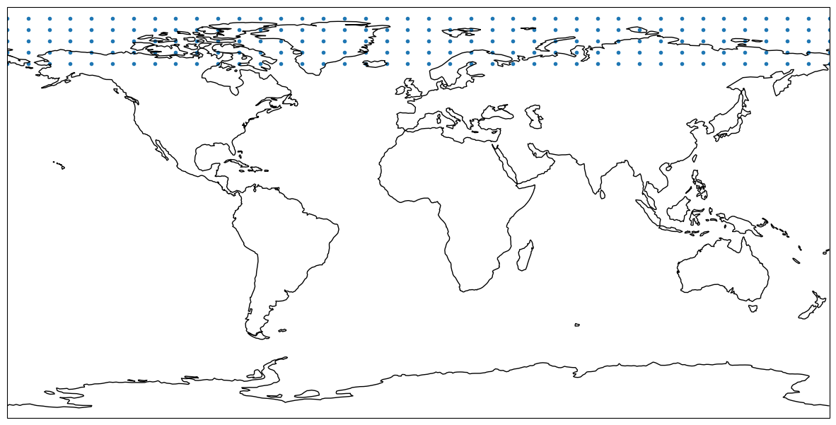
In the example below we create lat-lons laid out around the geographic North Pole. These example points are equidistantly spaced, but this does not have to be the case.
import numpy as np
import matplotlib.pyplot as plt
import cartopy.crs as ccrs

longitudes = np.linspace(-180, 180, 40)
latitudes = np.linspace(65, 85, 5)  # Very close to north pole

meshgridded_lat_lons = np.meshgrid(longitudes, latitudes)
coords = np.stack([mg_coord.flatten() for mg_coord in meshgridded_lat_lons], axis=1)

fig, ax = plt.subplots(figsize=(15, 9), subplot_kw={"projection": ccrs.PlateCarree()})
ax.scatter(coords[:, 0], coords[:, 1], marker=".")
ax.coastlines()
ax.set_extent((-180, 180, -90, 90))
/home/runner/work/weather-model-graphs/weather-model-graphs/.venv/lib/python3.12/site-packages/cartopy/io/__init__.py:242: DownloadWarning: Downloading: https://naturalearth.s3.amazonaws.com/110m_physical/ne_110m_coastline.zip
  warnings.warn(f'Downloading: {url}', DownloadWarning)
We first consider what happens if we directly feed these lat-lons as coords, treating them as if they were Cartesian coordinates. In this notebook we will only create flat “Keisler-like” graphs, but everything works analogously for the other graph types.
import weather_model_graphs as wmg

graph = wmg.create.archetype.create_keisler_graph(coords, mesh_node_distance=10)
fig, ax = plt.subplots(figsize=(15, 9), subplot_kw={"projection": ccrs.PlateCarree()})
wmg.visualise.nx_draw_with_pos_and_attr(
    graph, ax=ax, node_size=30, edge_color_attr="component", node_color_attr="type"
)
ax.coastlines()
ax.set_extent((-180, 180, -90, 90))
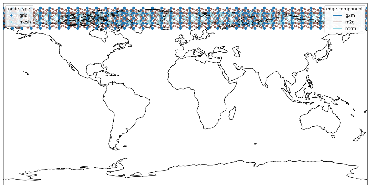
This creates a useable mesh graph, but we can note a few problems with it:
There are no connections between nodes around longitude -180/180, i.e. the periodicity of longitude is not considered.
All nodes at the top of the plot, close to the pole, are actually very close spatially. Yet there are no connections between them.
These are issues both in the connection between the grid nodes and the mesh, and in the connections between mesh nodes. This points to the fact that we should probably use a different projection when building our graph.
Constructing a graph within a projection#
For our example above, let’s instead try to construct the graph based on first projecting our lat-lon coordinates to another CRS with 2-dimensional cartesian coordinates. This can be done by giving the coords_crs and graph_crs arguments to the graph creation functions. Theses arguments should both be instances of pyproj.crs.CRS (pyproj docs.). Nicely, they can be cartopy.crs.CRS, which provides easy ways to specify such CRSs. For more advanced use cases a pyproj.crs.CRS can be specified directly. See the cartopy documentation for a list of readily available CRSs to use for projecting the coordinates.
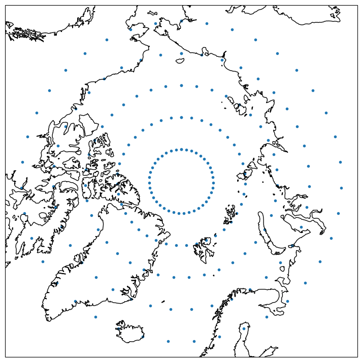
We will here try the same thing as above, but using a Azimuthal equidistant projection centered at the pole. The CRS of our lat-lon coordinates will be cartopy.crs.PlateCarree and we want to project this to cartopy.crs.AzimuthalEquidistant:
# Define our projection
coords_crs = ccrs.PlateCarree()
graph_crs = ccrs.AzimuthalEquidistant(central_latitude=90)

fig, ax = plt.subplots(figsize=(15, 9), subplot_kw={"projection": graph_crs})
ax.scatter(coords[:, 0], coords[:, 1], marker=".", transform=ccrs.PlateCarree())
_ = ax.coastlines()
/home/runner/work/weather-model-graphs/weather-model-graphs/.venv/lib/python3.12/site-packages/cartopy/io/__init__.py:242: DownloadWarning: Downloading: https://naturalearth.s3.amazonaws.com/50m_physical/ne_50m_coastline.zip
  warnings.warn(f'Downloading: {url}', DownloadWarning)
Note that distances within projections tend to have very large magnitudes, so the distance between mesh nodes should be specified accordingly.
mesh_distance = (
    10**6
)  # Large euclidean distance in projection coordinates between mesh nodes
graph = wmg.create.archetype.create_keisler_graph(
    coords, mesh_node_distance=mesh_distance, coords_crs=coords_crs, graph_crs=graph_crs
)  # Note that we here specify the projection argument
fig, ax = plt.subplots(figsize=(15, 9), subplot_kw={"projection": graph_crs})
wmg.visualise.nx_draw_with_pos_and_attr(
    graph, ax=ax, node_size=30, edge_color_attr="component", node_color_attr="type"
)
_ = ax.coastlines()
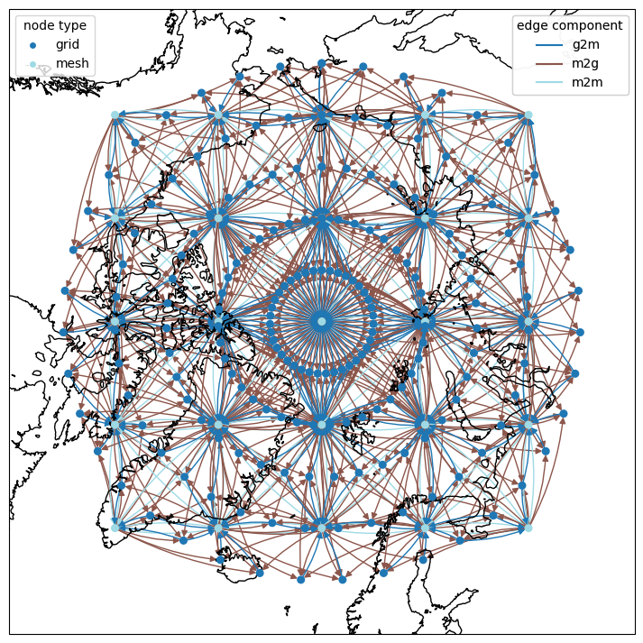
Now this looks like a more reasonable graph layout, that better respects the spatial relations between the grid points. There are still things that could be tweaked further (e.g. the large number of grid nodes connected to the center mesh node), but this ends our example of defining graphs using lat-lon coordinates.
It can be noted that this projection between different CRSs provides more general functionality than just handling lat-lon coordinates. It is entirely possible to transform from any coords_crs to any graph_crs using these arguments.