Creating the graph

Within graph-based weather models one single graph is used to represent the encode-process-decode operations of the data-driven weather model. The graph is a directed acyclic graph (DAG) with the nodes representing features at a given location in space and the edges representing flow of information.

weather-model-graphs provides a framework for creating and visualising graphs for data-driven weather models. The framework is designed to be flexible and allow for the creation of a wide range of graph architectures.

The graph is comprised of three components that represent the three encode-process-decode operations:

• g2m: The encoding from the physical grid space onto the computational mesh space.

• m2m: The processing of the data in the computational mesh space.

• m2g: The decoding from the computational mesh space onto the physical grid space.

The graph is a directed acyclic graph (DAG) with the nodes representing points in space and the edges

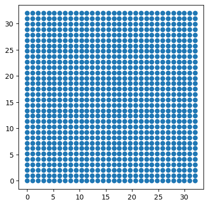
The grid nodes

To get started we will create a set of fake grid nodes, which represent the geographical locations where we have values for the physical fields. We will here work with cartesian x/y coordinates. See this page for how to use lat/lon coordinates in weather-model-graphs.

import numpy as np
import matplotlib.pyplot as plt
import weather_model_graphs as wmg

def _create_fake_xy(N=10):
    x = np.linspace(0.0, N, N)
    y = np.linspace(0.0, N, N)
    xy_mesh = np.meshgrid(x, y)
    xy = np.stack([mg_coord.flatten() for mg_coord in xy_mesh], axis=1)  # Shaped (N, 2)
    return xy

xy = _create_fake_xy(32)

fig, ax = plt.subplots()
ax.scatter(xy[:, 0], xy[:, 1])
ax.set_aspect(1)

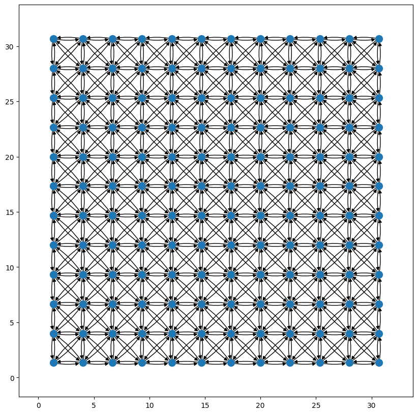
The mesh nodes and graph

Lets start with a simple mesh which only has nearest neighbour connections. At the moment weather-model-graphs creates a rectangular mesh that sits within the spatial domain spanned by the grid nodes (specifically within the axis-aligned bounding box of the grid nodes). Techniques for adding non-square meshes are in development.

g_m2m = wmg.create.mesh.create_single_level_2d_mesh_graph(xy=xy, nx=12, ny=12)

wmg.visualise.nx_draw_with_pos_and_attr(g_m2m)

<Axes: >

Graph archetypes

To simplify the creation of the full encode-process-decode graph, the weather-model-graphs package contains implementations of a number of graph archetypes. These architypes principally differ in the way the mesh component of the graph is constructed, but also in the way the grid and mesh components are connected. As more approaches are developed they will be added to the library.

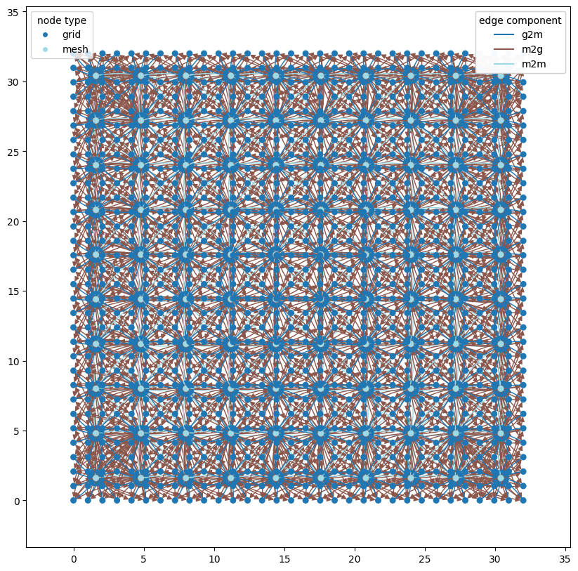
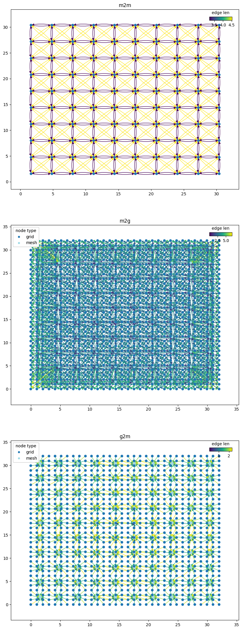
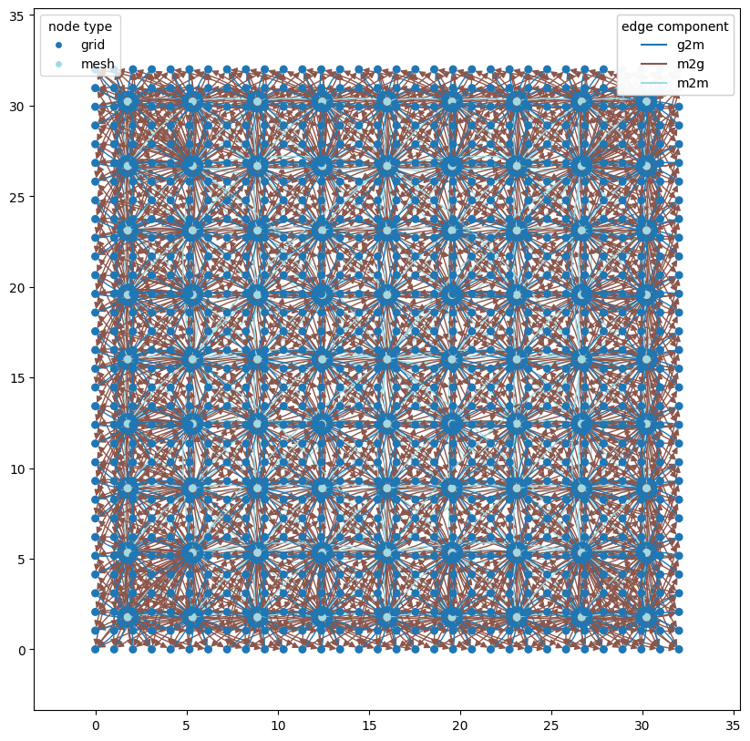
The Keisler 2022 single-range mesh

The first archetype is the single-range mesh from Keisler 2022 which demonstrated that graph-based neural-netwoks can be used to predict the weather with similar accuracy to traditional numerical weather models. The mesh is a simple nearest-neighbour mesh with a single range of connections.

?wmg.create.archetype.create_keisler_graph

graph = wmg.create.archetype.create_keisler_graph(coords=xy)
graph

<networkx.classes.digraph.DiGraph at 0x7f829207d6a0>

wmg.visualise.nx_draw_with_pos_and_attr(
    graph, node_size=30, edge_color_attr="component", node_color_attr="type"
)

<Axes: >

graph_components = wmg.split_graph_by_edge_attribute(graph=graph, attr="component")
graph_components

{'m2m': <networkx.classes.digraph.DiGraph at 0x7f829266f0b0>,
 'm2g': <networkx.classes.digraph.DiGraph at 0x7f82923183b0>,
 'g2m': <networkx.classes.digraph.DiGraph at 0x7f828788e3c0>}

n_components = len(graph_components)
fig, axes = plt.subplots(nrows=n_components, ncols=1, figsize=(10, 9 * n_components))

for (name, g), ax in zip(graph_components.items(), axes.flatten()):
    pl_kwargs = {}
    if name == "m2m":
        pl_kwargs = dict(edge_color_attr="len")
    elif name == "g2m" or name == "m2g":
        pl_kwargs = dict(edge_color_attr="len", node_color_attr="type")

    wmg.visualise.nx_draw_with_pos_and_attr(graph=g, ax=ax, node_size=30, **pl_kwargs)
    ax.set_title(name)

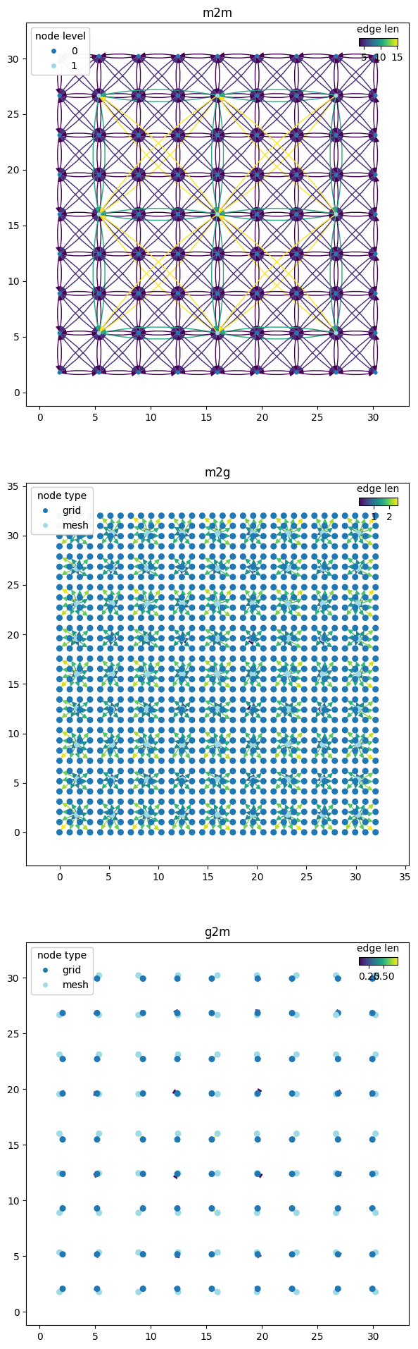
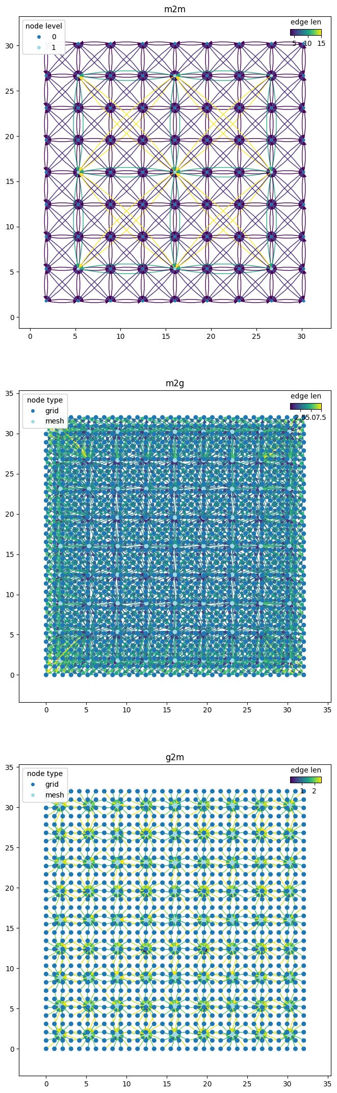
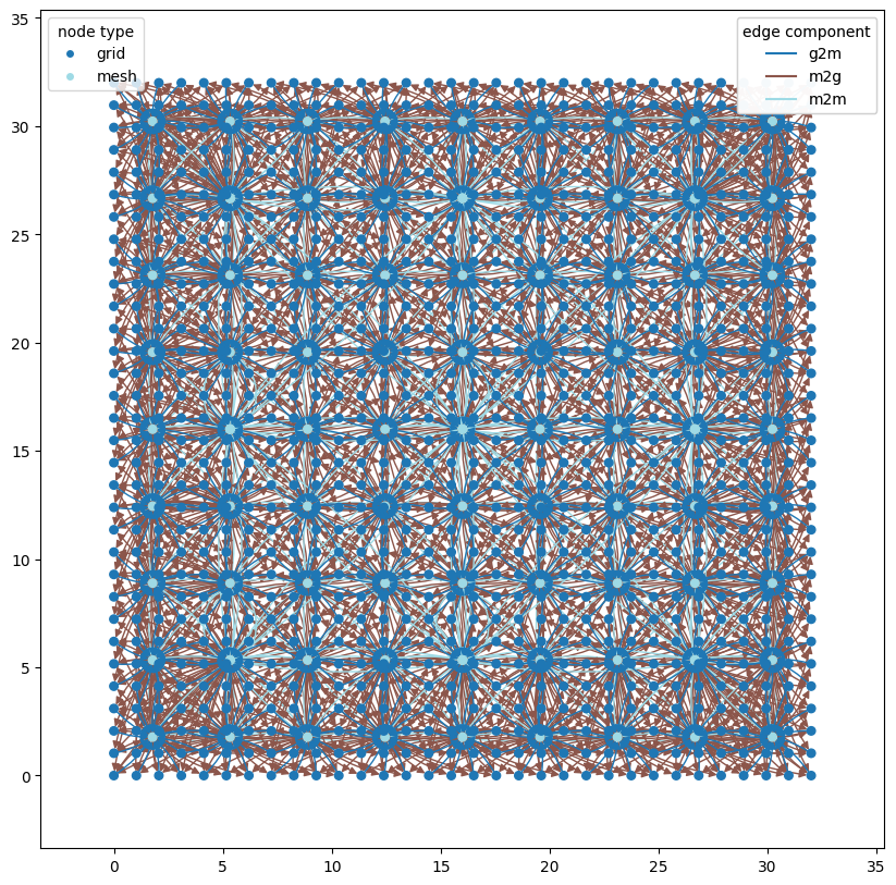
GraphCast (Lam et al 2022) graph

The second archetype is the GraphCast graph from Lam et al 2022 which built on the Keisler 2022 graph by adding longer-range connections in the mesh component of the graph. This allows the model to capture both short and long-range spatial interactions.

?wmg.create.archetype.create_graphcast_graph

graph = wmg.create.archetype.create_graphcast_graph(coords=xy)

wmg.visualise.nx_draw_with_pos_and_attr(
    graph, node_size=30, edge_color_attr="component", node_color_attr="type"
)

<Axes: >

graph_components = wmg.split_graph_by_edge_attribute(graph=graph, attr="component")
graph_components

{'m2m': <networkx.classes.digraph.DiGraph at 0x7f8280710470>,
 'm2g': <networkx.classes.digraph.DiGraph at 0x7f8283b8e6c0>,
 'g2m': <networkx.classes.digraph.DiGraph at 0x7f82921bf3b0>}

n_components = len(graph_components)
fig, axes = plt.subplots(nrows=n_components, ncols=1, figsize=(10, 9 * n_components))

for (name, g), ax in zip(graph_components.items(), axes.flatten()):
    pl_kwargs = {}
    if name == "m2m":
        pl_kwargs = dict(edge_color_attr="len", node_color_attr="level", node_size=10)
    elif name == "g2m" or name == "m2g":
        pl_kwargs = dict(edge_color_attr="len", node_color_attr="type", node_size=30)

    wmg.visualise.nx_draw_with_pos_and_attr(graph=g, ax=ax, **pl_kwargs)
    ax.set_title(name)
    ax.set_aspect(1.0)

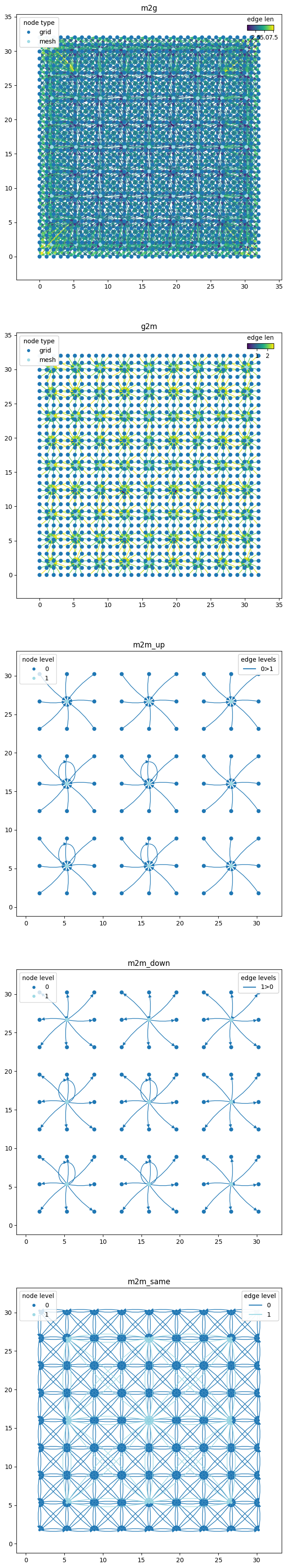
Oskarsson et al 2023 hierarchical graph

The hierarchical graph from Oskarsson et al 2023 builds on the GraphCast graph by adding a hierarchical structure to the mesh component of the graph. This allows the model to capture both short and long-range spatial interactions and to learn the spatial hierarchy of the data. The message-passing on different levels of interaction length-scales are learnt separately (rather than in a single pass) which allows the model to learn the spatial hierarchy of the data.

?wmg.create.archetype.create_oskarsson_hierarchical_graph

graph = wmg.create.archetype.create_oskarsson_hierarchical_graph(coords=xy)
graph

<networkx.classes.digraph.DiGraph at 0x7f8286cdc7d0>

wmg.visualise.nx_draw_with_pos_and_attr(
    graph, node_size=30, edge_color_attr="component", node_color_attr="type"
)

<Axes: >

The hierarchical graph is a bit more complex, so we will not only split by the g2m, m2m and m2g components, but also further split the m2m component into the different directions that the edges form in the hierarchical mesh graph. Specifically, the m2m graph component will be split into three: 1) m2m_up, 2) m2m_same and 3) m2m_down, using the utility function wmg.split_graph_by_edge_attribute(...) to use the direction attribute that each of the nodes in the m2m graph components has. This makes it possible to visualise each of these parts of the graph separately:

graph_components = wmg.split_graph_by_edge_attribute(graph=graph, attr="component")
m2m_graph = graph_components.pop("m2m")
# we'll create an identifier for each m2m component so that we know that what part of the
# m2m subgraph we're looking at
m2m_graph_components = {
    f"m2m_{direction}": graph
    for direction, graph in wmg.split_graph_by_edge_attribute(
        graph=m2m_graph, attr="direction"
    ).items()
}
graph_components.update(m2m_graph_components)
graph_components

{'m2g': <networkx.classes.digraph.DiGraph at 0x7f8286932fc0>,
 'g2m': <networkx.classes.digraph.DiGraph at 0x7f827cbae780>,
 'm2m_same': <networkx.classes.digraph.DiGraph at 0x7f827ca3b110>,
 'm2m_up': <networkx.classes.digraph.DiGraph at 0x7f827cc5d400>,
 'm2m_down': <networkx.classes.digraph.DiGraph at 0x7f827cac11f0>}

n_components = len(graph_components)
fig, axes = plt.subplots(nrows=n_components, ncols=1, figsize=(10, 9 * n_components))

for (name, graph), ax in zip(graph_components.items(), axes.flatten()):
    pl_kwargs = {}
    if name == "m2m_same":
        pl_kwargs = dict(edge_color_attr="level", node_color_attr="level", node_size=10)
    elif name == "g2m" or name == "m2g":
        pl_kwargs = dict(edge_color_attr="len", node_color_attr="type", node_size=30)
    elif name in ["m2m_up", "m2m_down"]:
        pl_kwargs = dict(
            edge_color_attr="levels", node_color_attr="level", node_size=30
        )

    wmg.visualise.nx_draw_with_pos_and_attr(graph, ax=ax, **pl_kwargs)
    ax.set_title(name)
    ax.set_aspect(1.0)

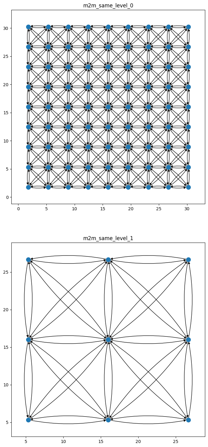
Finally, we can repeat this with the m2m_same graph and split by level, so that we can see the connections in each hiearchical level of the graph separately:

m2m_same_graph = graph_components["m2m_same"]
# we'll create an identifier for each m2m component so that we know that what part of the
# m2m subgraph we're looking at
m2m_same_graph_components = {
    f"m2m_same_level_{level}": graph
    for level, graph in wmg.split_graph_by_edge_attribute(
        graph=m2m_same_graph, attr="level"
    ).items()
}
m2m_same_graph_components

{'m2m_same_level_0': <networkx.classes.digraph.DiGraph at 0x7f8286c6f800>,
 'm2m_same_level_1': <networkx.classes.digraph.DiGraph at 0x7f827cac1e50>}

n_components = len(m2m_same_graph_components)
fig, axes = plt.subplots(nrows=n_components, ncols=1, figsize=(10, 9 * n_components))

for (name, graph), ax in zip(m2m_same_graph_components.items(), axes.flatten()):
    wmg.visualise.nx_draw_with_pos_and_attr(graph, ax=ax)
    ax.set_title(name)
    ax.set_aspect(1.0)

Creating your own graph architecture

Instead of creating one of the archetype above, you can also create your own graph architecture. This can be done by calling the create_all_graph_components function and defining the g2m, m2m and m2g connectivity method (any arguments for each).

Here we will only make nearest-neighbour connections in both directions between the mesh and grid nodes. As you will see below that leads to a graph that ignores most of the input from the grid nodes, so this is not a good graph architecture.

graph = wmg.create.create_all_graph_components(
    m2m_connectivity="flat_multiscale",
    coords=xy,
    m2m_connectivity_kwargs=dict(
        mesh_node_distance=2, level_refinement_factor=3, max_num_levels=None
    ),
    g2m_connectivity="nearest_neighbour",
    m2g_connectivity="nearest_neighbour",
)

graph_components = wmg.split_graph_by_edge_attribute(graph=graph, attr="component")

fig, axes = plt.subplots(nrows=3, ncols=1, figsize=(8, 24))

for (name, graph), ax in zip(graph_components.items(), axes.flatten()):
    pl_kwargs = {}
    if name == "m2m":
        pl_kwargs = dict(edge_color_attr="len", node_color_attr="level", node_size=10)
    elif name == "g2m" or name == "m2g":
        pl_kwargs = dict(edge_color_attr="len", node_color_attr="type", node_size=30)

    wmg.visualise.nx_draw_with_pos_and_attr(graph, ax=ax, **pl_kwargs)
    ax.set_title(name)
    ax.set_aspect(1.0)